Rune Linding1†*, Lars Juhl Jensen12†, Francesca Diella3, Peer Bork12, Toby J. Gibson1 and Robert B. Russell1
† These authors contributed equally.
* To whom correspondence should be addressed (email: linding@embl.de)
IDPs - Intrinsically Disordered Proteins
ELMs - Eukaryotic Linear Motifs
PONDR - Predictor Of Natural Disordered Regions
B-factors - atomic displacement parameters; temperature factors
PDB - Protein databank
DSSP - Dictionary of Secondary Structure of Proteins
protein disorder; intrinsic disorder; hot loops; target selection; structural genomics; structural biology; structural proteomics
A great challenge in the proteomics and structural genomics era is to predict protein structure and function, including identification of those proteins that are partially or wholly unstructured. Disordered regions in proteins often contain short linear peptide motifs (e.g. SH3-ligands and targeting signals) that are important for protein function. We present here DisEMBL, a computational tool for prediction of disordered/unstructured regions within a protein sequence. As no clear definition of disorder exists, we have developed parameters based on several alternative definitions, and introduced a new one based on the concept of "hot loops", i.e. coils with high temperature factors. Avoiding potentially disordered segments in protein expression constructs can increase expression, foldability and stability of the expressed protein. DisEMBL is thus useful for target selection and the design of constructs as needed for many biochemical studies, particularly structural biology and structural genomics projects. The tool is freely available via a web interface (http://dis.embl.de) and can be downloaded for use in large scale studies.
In the post-genomic era, discovery of novel domains and functional sites in proteins is of growing importance. One focus of structural genomics initiatives is to solve structures for novel domains and thereby increase the coverage of fold and structure space (Brenner, 2000). During the target selection process in structural genomics/biology intrinsic protein disorder is important to consider since disordered regions at the N- and C- termini (or even within domains) often leads to difficulties in protein expression, purification and crystallisation. It is therefore essential to be able to predict which regions of a target protein are potentially disordered/unstructured. Computational tools to help discern ordered globular domains from disordered regions are key to such efforts.
It is becoming increasingly clear that many functionally important protein segments occur outside of globular domains (Wright and Dyson, 1999 and Dunker et al., 2002). Protein structure and function space is partitioned in two sub spaces. The first consist of globular units with binding pockets, active sites and interaction surfaces. The second sub space contains non-globular segments such as sorting signals, post-translational modification sites and protein ligands (e.g. SH3 ligands). Globular units are built of regular secondary structure elements and contribute the majority of the structural data deposited in PDB. In contrast, the non-globular sub space encompasses disordered, unstructured and flexible regions without regular secondary structure. Functional sites within the non-globular space are known as linear motifs (catalogued by ELM, http://elm.eu.org) (Puntervoll et al., 2003).
There are also many recent reports of Intrinsically Disordered Proteins (IDPs, also known as Intrinsically Unstructured Proteins). These are proteins or domains that, in their native state, are either completely disordered or contain large disordered regions. More than 100 such proteins are known including Tau, Prions, Bcl-2, p53, 4E-BP1 and eIF1A (see Figure 4) (Tompa, 2002 and Uversky, 2002).
Protein disorder is important for understanding protein function as well as protein folding pathways (Plaxco and Gross, 2001 and Verkhivker et al., 2003). Although little is understood about the cellular and structural meaning of IDPs, they are thought to become ordered only when bound to another molecule (e.g. CREB-CBP complex (Radhakrishnan et al., 1997)) or owing to changes in the biochemical environment (Dunker et al., 2001, Dunker et al., 2002, and Uversky, 2002).
The current view on disorder is that disordered proteins are disordered to allow for more interaction partners and modification sites (Wright and Dyson, 1999, Liu et al., 2002, and Tompa, 2002). It has also been suggested that disordered proteins exist to provide a simple solution to having large intermolecular interfaces while keeping smaller protein, genome and cell sizes (Gunasekaran et al., 2003). It has been noted that having several relatively low affinity linear interaction sites allows for a flexible, subtle regulation as well as account for specificity with fewer linear motifs types (Evans and Owen, 2002). It has also been demonstrated that protein disorder plays a central role in biology and in diseases mediated by protein misfolding and aggregation (Schweers et al., 1994, Kaplan et al., 2003, and Bates, 2003).
No commonly agreed definition of protein disorder exists. The thermodynamic definition of disorder in a polypeptide chain is the "random coil" structural state. The random coil state can best be understood as the structural ensemble spanned by a given polypeptide in which all degrees of freedom are used within the conformational space. However, even under extremely denaturing solvation conditions, such as 8M urea, this theoretical state is not observed in solvated proteins (Shortle and Ackerman, 2001, Ackerman and Shortle, 2002, and Klein-Seetharaman et al., 2002). Proteins in solution thus seem to always keep a certain amount of residual structure.
Protein disorder is only indirectly observed by a variety of experimental methods, such as X-ray crystallography, NMR-, Raman-, CD-spectroscopy and hydrodynamic measurements (Smyth et al., 2001 and Dunker et al., 2001). In vivo studies of disorder are possible with NMR spectroscopy on living cells (e.g. anti-sigma factor FlgM (Dedmon et al., 2002)). Each one of these methods detects different aspects of disorder resulting in several operational definitions of protein disorder (see Tompa, 2002 for a review).
There have been several previous attempts to predict disorder. Perhaps the earliest are methods finding regions of low-complexity. Although many such regions are structurally disordered, the correlation is far from perfect as regions of low sequence complexity are not always disordered (and vice versa) (Dunker et al., 2002). Likely the strongest evidence for this correlation comes from the fact that low-complexity regions are rarely seen in protein 3D structures (Saqi and Sternberg, 1994). Methods to predict low complexity, like SEG (Wootton, 1994) and CAST (Promponas et al., 2000), are thus often used for this purpose. Methods using hydrophobicity can also give hints as to disordered regions, as they are typically exposed and rarely hydrophobic.
The first tool designed specifically for prediction of protein disorder was PONDR (Predictor Of Naturally Disordered Regions, http://www.pondr.com) (Romero et al., 1997, Garner et al., 1998, and Garner et al., 1999). It is based on artificial neural networks. An alternative method is GlobPlot (http://globplot.embl.de) that instead relies on a novel propensity based disorder prediction algorithm (Linding et al., 2003).
Regions without regular secondary structure can be predicted by the NORSp (NOn Regular Structure) server (Liu et al., 2002), however as the authors admit such regions are not necessarily disordered. Structures such as the Kringle domain (PDB: 1KRN) are almost entirely without regular secondary structure in their native state but they still have tertiary structure wherein the basic building block is coils. These "loopy proteins" are not necessarily IDPs since they can still form a well defined globular tertiary structure.
Prediction of protein tertiary structure could be an alternative route to disorder prediction, though such methods are computationally intensive and error-prone. Moreover such methods are usually designed to predict the structure of globular domains, meaning that their behaviour on other sequences can be unpredictable.
Here we present DisEMBL a method based on artificial neural networks trained for predicting several definitions of disorder. It predicts and displays the probability of disordered segments within a protein sequence. DisEMBL furthermore provide a pipeline interface for bulk predictions, essential for large scale structural genomics.
As no single definition of disorder exists, we will describe in detail what we define as disordered regions. We describe protein disorder as two-state models where each residue is either ordered or disordered. For this purpose we used three different criteria for assigning disorder:
A fundamental problem with X-ray data, is that it is limited to what is found in the PDB. Many structures are solved on truncated polypeptides, explicitly because the parts that are cut off are disordered or highly flexible, meaning that the data set itself is truncated. Some of these regions could be recovered by combining PDB with sequence databases, however this cannot be performed in an automated fashion.
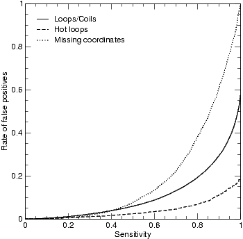
Sensitivity and rate of false positives for the various DisEMBL neural networks. The receiver output characteristic (ROC) curves were constructed from cross validation test set performances. Performances are reported on a per residue basis. Since the data sets were homology reduced based on SCOP, the performances shown correspond to what can be expected for novel protein sequences.
For each of the three definitions of disorder described above, a data set was constructed and partitioned into five cross validation sets. We trained an ensemble of five artificial neural networks on each the three data sets. Figure 1 shows the expected performance for these three predictors on novel sequences as estimated by cross validation. As can be seen, we are able to predict a large fraction of the missing coordinate residues with a very low error rate.
The coils networks predict regions without regular secondary structure: it is a two state secondary structure prediction method. This neural network ensemble is capable of identifying approximately half of the negative examples, while discarding essentially no positive examples (see Figure 1). Therefore this predictor is perhaps better thought of as a filter to remove false positive predictions made by the other networks.
Separate networks were trained for predicting which of the loops have high B-factors ("hot loops"). The performance of these networks are shown in Figure 1. Hot loops are predicted using these two network ensembles collectively. The overall performance of this composite predictor can be estimated from the individual performances of these ensembles as follows. Choosing a cutoff of 80% sensitivity for each ensemble corresponds to a sensitivity of 64% (80%*80%) for the composite predictor. At these cutoffs the rate of false positives are 6.9% and 19% respectively, corresponding to 1.3% then combined. It follows that hot loops are very predictable. In contrast, the missing coordinates predictor has a higher (16%) rate of false positives at the same sensitivity. A possible explanation for this is that REMARK465 can be assigned to a residue for several reasons, disorder being only one of these.
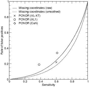
Comparison with PONDR. We tested the performance of our networks the data sets from Dunker et al (http://disorder.chem.wsu.edu/PONDR/PONDR.htm). Only the performance points for the various PONDR predictors reported at the web site are shown, as we do not have access to the raw PONDR predictions. Relative to these points, the REMARK465 predictor of DisEMBL, performs marginally better than PONDR.
We compared DisEMBL to PONDR, refer to Figure 2. The comparison to PONDR was severely hampered by the fact that access to raw PONDR predictions is restricted. Therefore we can currently only compare to the performance points stated on the official website of PONDRs developers. Since the VL-XT predictor is smoothing its predictions by a running average of 9 residues, we also applied this smoothing to our predictions. Relative to these points our predictor performs marginally better in predicting the same type of disorder. We only use smoothing in this comparison as the performance gain is a consequence of the design of this particular data set. Smoothing does not improve performance on our own data sets.
In order to investigate the relationships between the different disorder definitions we determined how correlated our predictors are. This was done by calculating the linear Pearson correlation coefficients for the predictions by the three predictors on a data set consisting of one sequence from each protein family in SCOP version 1.61. The correlation between hot loops and coils is trivial since the data set used for training the hot loop predictor is a sub set of the one used for the coils network. The predictions of missing coordinates and coils are only weakly related (CC = 0.231), while the hot loops predictions show a stronger correlation to the REMARK465 networks (CC = 0.455).
Since we initially assumed that missing coordinates directly reflects protein disorder the correlation with the hot loops predictions support this alternative definition of disorder, it also shows that the definitions are complementary not redundant.
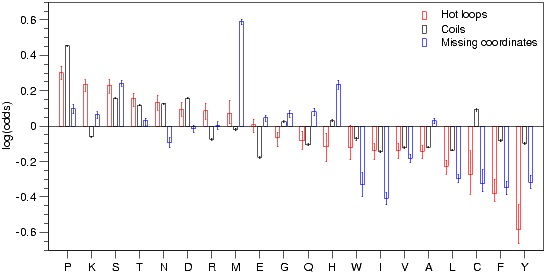
Propensities for the amino acids to be disordered according to the three definitions used in this work (sorted by hot loop preference). This scale is directly reflecting what was in the data sets used for training, however it is only a first approximation of what the neural networks are using in predicting disorder. The coils scale is similar to the Russell/Linding propensity scale described in (Linding et al., 2003). Error bars correspond to the 25 and 75 percentiles as estimated by stochastic simulation.
The relationship between the different predictors can also be seen in Figure 3. The figure shows the per residue counts in the different data sets. In general hydrophobic residues are promoting order according to all three definitions of disorder. Disorder promoting residues include proline, lysine, serine, threonine and methionine. For lysine it can be seen that even though this residue is not observed much in coils it is found primarily in hot loops, the opposite is the case for proline. Methionine suffers a bias in the REMARK465 dataset for at least two reasons: 1) often the N-terminal methionine is cleaved off 2) some structures are solved using selenomethionine derivatives for phasing, which can lead to deletion of the residue in the PDB entry. The same bias is seen in Dunker et al., 2001 Figure 10.
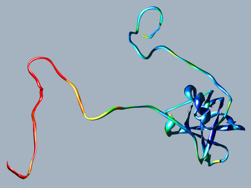
DisEMBL hot loop predictions mapped on the NMR mean structure of human translation initiation factor eIF1A (PDB: 1D7Q, SWISS-PROT: P47813). The predicted probabilities were with a colour scale going from blue to red, where red corresponds to the most likely disordered regions and blue to ordered regions. Both the manually assigned disordered regions score higher than the globular domain, in particular the N-terminal one (Battiste et al., 2000).
As mentioned NMR and CD data can provide insight on protein disorder. Since such data were not used during training, they provide good examples for validating our predictors. NMR parameters such as order vectors, chemical shifts within the "random coil window" and disordered residues as assigned by the authors, will likely provide the best data sets for training disorder predictors in the future. Chemical shifts are already being used for prediction of secondary structure and coils, e.g. in TALOS (Cornilescu et al., 1999). Unfortunately, NMR data are rather scarce and only cover a subset of structure space, which is why we have not used such data for training predictors. However, it is interesting to notice that our predictions of disordered regions seem to agree with disorder determined by NMR. An example of this is Figure 4, which shows predictions of hot loops mapped on the NMR structure of human translation factor eIF1A.
Missing signals in the far UV of CD spectra indicate the absence of regular secondary structure. A fundamental problem in using CD data for assigning disorder is that the lack of regular secondary structure does not imply that the protein is disordered, merely that it is a "loopy protein". Another disadvantage of CD data is that they do not provide information on which residues are disordered. The same limitations apply to hydrodynamic measurements. We have therefore not used CD or hydrodynamic data in the training of our predictors.
| Protein (acc number) | DisEMBL hot loops segments |
Protein length |
|---|---|---|
| Histone H1.2 (P15865) | 1-39 110-218 | 218 |
| Samatolliberin(GHRH) (P42692) | 1-4 28-45 | 45 |
| Protamine (P15340) | 1-61 (full length) | 61 |
| CREB (P15337) | 1-10 100-170 330-341 | 341 |
| 30S Ribosomal Protein (P02379) | 1-70 (full length) | 70 |
| Prothymosin alpha (P01252) | 1-109 (full length) | 109 |
| cAMP-dependent PKI (P04541) | 1-20 26-34 50-75 | 75 |
| Hirudin (P01050) | 1-13 42-65 | 65 |
Hot loops predictions on proteins that are reported to be IDPs according to CD data (Tompa, 2002, Uversky, 2002, and Dunker et al., 2001).
However, the lack of residue specific information allows us to make predictions of disordered segments within proteins shown to contain such segments by CD. A number of examples previously described in the literature as being disordered were analysed with DisEMBL (Table 1). In all of these cases, we predict either all or large parts of the protein to be disordered. In the case of histone H1.2 the predictions are in agreement with what is known from experimental studies of the homologue histone H5 and other linker histones (Aviles et al., 1978). CREB is another that has been intensively studied, we correctly predict the unstructured pKID domain (approx. residues 113-154) (Radhakrishnan et al., 1997, Wright and Dyson, 1999, and Demarest et al., 2002).
The DisEMBL prediction method is publicly accessible as a web server at http://dis.embl.de for predicting disorder in proteins. Although the GlobPlot server at http://globplot.embl.de can also be used for predicting protein disorder, the two methods complement each other as they approach disorder prediction differently. GlobPlot is less accurate than DisEMBL in coils prediction, however it was designed as a visual inspection tool for finding both domain boundaries, repeats and unstructured regions. Furthermore, the GlobPlot algorithm is very simple and intuitive, which might appeal to some users.
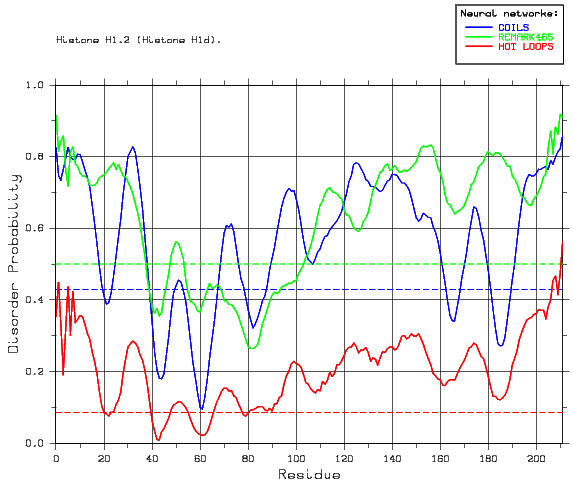
Sample output from the DisEMBL web server, showing predictions for Histone H1.2 (P15865). The green curve is the predictions for missing coordinates, red for the hot loop network and blue for coil. The horizontal lines correspond to the random expectation level for each predictor; for coils and hot loops the prior probabilities were used, while a neural network score of 0.5 is used for REMARK465. From this plot it is seen that the predictors agree on residues 1-39 and 110-218 as being disordered.
The web interface is fairly straight forward to use, the user can paste a sequence or enter the SWISS-PROT/SWALL accession (e.g. P08630) or entry code (e.g. PRIO_HUMAN). The DisEMBL server fetches the sequence and description of the polypeptide from an ExPASy server using Biopython.org software. The probability of disorder is shown graphically, as illustrated at Figure 5. The random expectation levels for the different predictors are shown on the graph as horizontal lines but should only be considered an absolute minimum.
The user will normally not have to change the default parameters, but on line documentation of the different settings are provided at http://dis.embl.de/help.html. If the query protein sequence is very long, >1000 residues, the user can download the predictions and use a local graph/plotting tool such as Grace or OpenOffice.org to plot and zoom the data.
Having identified the potential disordered regions, the user should now have a good basis for setting up expression vectors and/or comparing the data with obtained structural data. It is currently impossible to say which of the definitions of disorder is most appropriate for design of protein expression vectors. We thus strongly encourage feedback on successes and failures in using DisEMBL for expression and structural analysis of proteins.
The web server only allows predictions on one sequence at a time, if bulk predictions are needed we supply DisEMBL as a pipeline software package. The pipeline consists of the same three neural networks implemented as one ANSI C code module, which reads sequence from STDIN and writes predictions to STDOUT. The pipeline interface is intended for the structural genomics initiatives. The pipeline can analyse in the order of 1 million residues/min on a 1GHz x86 PC. This allows for very large scale predictions, e.g. as part of a structure space scanning. DisEMBL is released as OSI (http://www.opensource.org) certified opensource software and can be downloaded from http://dis.embl.de/download.html.
We have presented a method to predict disordered regions within protein sequences. Our method profits from predicting protein disorder according to multiple definitions, including the new concept of "hot loops". Furthermore, the method is highly accurate, predicting more than 60% of hot loops with less than 2% false positives. We anticipate that DisEMBL will be of great use to experimental biologists wishing to optimise constructs for expression and crystallisation, or who wish to identify features within a studied protein sequence. We expect further progress to come from a deeper understanding of disordered proteins, which will lead to more systematic definitions of the phenomenon.
The coils data set was constructed based on DSSP (Kabsch and Sander, 1983) secondary structure assignments as described in Linding et al., 2003. This data set only contains one chain from each SCOP superfamily according to SCOP 1.59. Two different versions of this data set were used for training neural networks. One version simply consists of the "raw" labeling of residues as described above, while the other version is filtered to only include regions of at least 7 consecutive residues with the same labeling. The latter version of the data set consists of 1238 sequences with 132395 labeled residues, 75424 of which are labeled as coil.
A second data set was constructed for discriminating between ordered and disordered loops. Loops were identified in a similar manner as in coil data set, only the Continuous DSSP (Andersen et al., 2002) rather than DSSP was used for secondary structure assignment and SCOP 1.61 was used for reducing the data set to one chain per family. As B-factors from different chains are not directly comparable, B-factors from regions of regular secondary structure were used for normalisation by establishing chain specific cutoffs for discriminating between ordered and disordered regions. Subsequently, all loop regions with B-factors below the median for secondary structure elements were labeled as ordered loops, while only those above the 90% fractile were considered to be disordered loops. This results in 1412 sequences containing only 795 residues labeled as being disordered.
Finally, a data set was constructed for the prediction of missing coordinates (REMARK465). Like the B-factor data set, this set was reduced to include only one chain from each protein family in to SCOP version 1.61 a total of 1547 sequences.
To form separate test and training sets, each of these data sets were split into five cross-validation partitions. As the data sets have already been reduced to at most one sequence per SCOP family, sequence similarity within the data set does not present a problem. Note that the use of single representatives from SCOP families ensures that no sequence detectable homologues are in the data set. Cross-validation performance estimates are thus independent of how the data sets are partitioned. To ensure that the partitions were balanced in the sense that each contains roughly the same number of disordered residues, the sequences were first sorted according to their number of disordered residues and then assigned to the five cross-validation partitions in a round-robin scheme.
Artificial neural networks were trained on symmetric sequence windows centered at the position to be predicted. All neural networks were trained with a learning rate of 0.005. The size of these windows was systematically varied from 3 to 51 residues. For each window size the number of hidden units was varied in the range 5-50. The performance of every such combination was evaluated by five fold cross validation and best parameter combinations were selected based on ROC curves.
The best cross-validation performance for the coil data set was obtained using the filtered version where only consistently labeled regions of at least 7 residues were considered. The optimal network architecture was a window size of 19 residues and 30 hidden units. Other networks with good performance all had similar network architectures and gave very similar predictions. No significant improvement in performance could thus be obtained by forming a larger ensemble of networks.
Separate networks were trained for the task of discriminating between ordered and disordered hot loops. Possibly because of the small number of positive examples, networks with many hidden neurons performed no better than those with few. This was especially true when using large window sizes. The best performing ensemble of networks had a window size of 41 residues and only 5 hidden neurons.
For prediction of missing coordinates (REMARK465) it was discovered that networks with a window size of 9 residues performed best at relatively low sensitivities while networks with a window size of 21 performed better for higher sensitivities; for both window sizes, 30 hidden units gave the best performance. An ensemble was thus formed consisting of two sets of five cross validation networks with window sizes of 9 and 21 residues respectively. This ensemble outperformed both the individual cross validation ensembles over the entire range of sensitivities.
The coil and hot loops neural network ensembles, the score distributions of positive and negative test examples were estimated using Gaussian kernel density estimation. Based on these distributions a calibration curve for converting neural network output scores to probabilities was constructed as previously described (Jensen et al., 2002). For coil prediction a prior probability of 43% (the composition of the training data set) was used while a prior probability of 20% was used in the case of hot loop prediction. As the resulting calibration curves were essentially linear, they were approximated by a least squares linear fit (corr. >0.99).
We run a digital low-pass filter based on Savitzky-Golay (refer to Press et al., 2002 section 14.8) on the network output in order to smooth the curves. The filtering is performed by an external open source C module (sav_gol) from the TISEAN 2.1 (Hegger et al., 1999) Nonlinear Time Series Analysis package (http://www.mpipks-dresden.mpg.de/~tisean/). The resulting smoothed functions are plotted using the DISLIN 8.0 package. DISLIN is distributed as platform specific binaries from http://www.linmpi.mpg.de/dislin/.
This work was partly supported by EU grant QLRI-CT-2000-00127. All neural networks used for this study were trained using the HOW program by Prof. Søren Brunak. Lars Juhl Jensen is funded by the Bundesministerium für Forschung und Bildung, BMBF-01-GG-9817. Thanks to Sophie Chabanis-Davidson and Sara Quirk for commenting on this manuscript. Finally we are deeply grateful to FreeBSD.org, (bio)Python.org, PostgreSQL.org, Debian.org and Apache.org for fantastic open free software.
Plaxco, K. W. and Gross, M. (2001). Unfolded, yes, but random? never! Nat. Struct. Biol., 8:659-660.
Tompa, P. (2002). Intrinsically unstructured proteins. Trends Biochem. Sci., 27:527-533.

